Calculate a weighted average

To do this task, use the SUMPRODUCT and SUM functions.
This example calculates the average price paid for a unit across three purchases, where each purchase is for a different number of units at a different price per unit.

	A	B
	Price per unit	Number of units
1	20	500
2	25	750
3	35	200
	Formula	Description (Result)
	=SUMPRODUCT(A2:A4,B2:B4)/SUM(B2:B4)	Divides the total cost of all three orders by the total number of units ordered (24.66)

This post is brought to you from the microsoft website

Excel Cell Formating

Today I would like to present you some tips on excel formatting; 1. Formatting an excel cell to Text, Number, Date , Time, Currency, Accounting, special or custom.         Select any excel cell and then on the menu click on Format then click on cell you can also use shortcut to open the cell formatting box directly by holding Ctrl+1 key, as shown in the following figure.    As in the above figure you can see Category box from where you can change the cell format to your desired format. You can do lot more than format in an excel cell. Make your excel cell a digital clock or digital image viewer, whatever you want just imagine and do it by using all the advanced features of cell formatting  to know more about how to do it just give a comment to this post.

Excel Drop Down List

Excel is excellent and lets see how it helps you using this drop down list features !
If you don't want to risk an item being miss-typed in a cell, drop down lists are an ideal solution. So These lists display all of the available choices to the user so that they can click on their preference. Excel allows you to place two different types of drop down list on your worksheet - either a validation list or a form object.
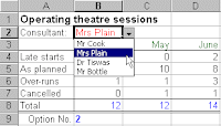
A validation drop down list
These lists are contained within a cell on your worksheet and the drop down arrow (to the right of the cell) does not appear unless the cell is selected. To add a list to a worksheet place the cursor in the required cell and then selectData Validation Settings. In the dialog box select 'Allow: List' and ensure the 'In-cell dropdown' box is ticked. The source data refers to a range of cells containing the selection of options. If you use the mouse to point to a range of cells (e.g. H12:H15), they must normally be contained on the same worksheet. If however you have named the range of cells (e.g. '=ConsNames') containing your data, it can be anywhere in the workbook.
In the example (right) the list has been placed in cell B2. Having selected 'Mrs Plain' the formulae in the table (B3:D8) lookup values in a range of data and summarise it. The consultant name can be referred to by the cell name (B2). If you wish to know the position of the selected item within the original range of options (i.e. the four names), an additional formula is needed. In cell B9, the formula =MATCH(B2, H12:H15, 0) determines that Mrs Plain is the second item in the list.

Using a combo box or a list box

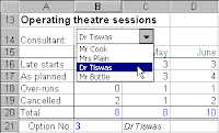
These are independent objects (or controls) that can be placed onto a worksheet and are not contained within a cell as such. The example (left) contains a combo box but your choice of object can depend on the amount of space on your worksheet and the number of options.

To obtain these controls you must open the Forms toolbar (View Toobars Forms). Then click on either of the list buttons and drag an outline for the object on your worksheet. To instruct the new control where to find it's source data, right click on it, then choose Format Controlfrom the short menu. On the 'Control' tab of the dialog box, enter the range of cells containing the list options. The 'Cell Link' refers to a cell where you wish the list box to place a numeric value representing selected item. In the example above cell B21 is linked and indicates that the third list item was selected. You cannot refer directly to the value in the list box, but the option number in your worksheet cell is automatically updated to reflect any change in the control object.
To determine the actual name of the selected item (i.e. Dr Tiswas), use a formula such as =OFFSET(H11, B21, 0) where H11 is the cell immediately above the options list and B21 contains the option value. (Click here for details about the OFFSET function).

credit:www.meadinkent.co.uk

Getting words from figures is excellent in excel

Amazing attribute of ms excel you can get your figures converted to words is as easy as 123. Only simple thing you got to know is this.....

------------------------------------------------------------------------------------
here is the formula!! you can copy this formula directly from here !!
---------------------------------------------------------------------------------------
Function ConvertCurrencyToEnglish(ByVal MyNumber) Dim Temp Dim Rupees, Paise Dim DecimalPlace, Count
ReDim Place(9) As String Place(2) = " Thousand " Place(3) = " Million " Place(4) = " Billion " Place(5) = " Trillion "
' Convert MyNumber to a string, trimming extra spaces. MyNumber = Trim(Str(MyNumber))
' Find decimal place. DecimalPlace = InStr(MyNumber, ".")
' If we find decimal place... If DecimalPlace > 0 Then ' Convert Paise Temp = Left(Mid(MyNumber, DecimalPlace + 1) & "00", 2) Paise = ConvertTens(Temp)
' Strip off Paise from remainder to convert. MyNumber = Trim(Left(MyNumber, DecimalPlace - 1)) End If
Count = 1 Do While MyNumber <> "" ' Convert last 3 digits of MyNumber to English Rupees. Temp = ConvertHundreds(Right(MyNumber, 3)) If Temp <> "" Then Rupees = Temp & Place(Count) & Rupees If Len(MyNumber) > 3 Then ' Remove last 3 converted digits from MyNumber. MyNumber = Left(MyNumber, Len(MyNumber) - 3) Else MyNumber = "" End If Count = Count + 1 Loop
' Clean up Rupees. Select Case Rupees Case "" Rupees = "" Case Else Rupees = " Rupees " & Rupees End Select
' Clean up Paise. Select Case Paise Case "" Paise = " " Case Else Paise = " and " & Paise & " Paise" End Select
ConvertCurrencyToEnglish = Rupees & Paise If Trim(ConvertCurrencyToEnglish) <> "" Then ConvertCurrencyToEnglish = ConvertCurrencyToEnglish & " Only" End Function
Private Function ConvertHundreds(ByVal MyNumber) Dim Result As String
' Exit if there is nothing to convert. If Val(MyNumber) = 0 Then Exit Function
' Append leading zeros to number. MyNumber = Right("000" & MyNumber, 3)
' Do we have a hundreds place digit to convert? If Left(MyNumber, 1) <> "0" Then Result = ConvertDigit(Left(MyNumber, 1)) & " Hundred " End If
' Do we have a tens place digit to convert? If Mid(MyNumber, 2, 1) <> "0" Then Result = Result & ConvertTens(Mid(MyNumber, 2)) Else ' If not, then convert the ones place digit. Result = Result & ConvertDigit(Mid(MyNumber, 3)) End If
ConvertHundreds = Trim(Result) End Function
Private Function ConvertTens(ByVal MyTens) Dim Result As String
' Is value between 10 and 19? If Val(Left(MyTens, 1)) = 1 Then Select Case Val(MyTens) Case 10: Result = "Ten" Case 11: Result = "Eleven" Case 12: Result = "Twelve" Case 13: Result = "Thirteen" Case 14: Result = "Fourteen" Case 15: Result = "Fifteen" Case 16: Result = "Sixteen" Case 17: Result = "Seventeen" Case 18: Result = "Eighteen" Case 19: Result = "Nineteen" Case Else End Select Else ' .. otherwise it's between 20 and 99. Select Case Val(Left(MyTens, 1)) Case 2: Result = "Twenty " Case 3: Result = "Thirty " Case 4: Result = "Forty " Case 5: Result = "Fifty " Case 6: Result = "Sixty " Case 7: Result = "Seventy " Case 8: Result = "Eighty " Case 9: Result = "Ninety " Case Else End Select
' Convert ones place digit. Result = Result & ConvertDigit(Right(MyTens, 1)) End If
ConvertTens = Result End Function
Private Function ConvertDigit(ByVal MyDigit) Select Case Val(MyDigit) Case 1: ConvertDigit = "One" Case 2: ConvertDigit = "Two" Case 3: ConvertDigit = "Three" Case 4: ConvertDigit = "Four" Case 5: ConvertDigit = "Five" Case 6: ConvertDigit = "Six" Case 7: ConvertDigit = "Seven" Case 8: ConvertDigit = "Eight" Case 9: ConvertDigit = "Nine" Case Else: ConvertDigit = "" End Select End Function
--------------------------------------------------------------------------------------
You have to paste this formula in a module in an excel sheet. Please check the below image
---------------------------------------------------------------------------------

Click here to download sample file:

When should you use the Vlookup function?

When you have a table with data, and you wish to retrieve specific information from it.
For example:You have an Excel table with student names and their grades.You wish that you could somewhere in the sheet type a student name, and immediately retrieve his grade (based on the data in the table).To achieve this, you can use "Vlookup": the function will look for the student’s name in the first column in the table, and will retrieve the information that is next to his name in the second column (which is his grade).
Another example:You have a big table consisting thousands of bank accounts.You wish to retrieve in another worksheet information regarding some specific accounts.To achieve this, you can type these specific account numbers, and put a Vlookup function next each one of them. The function will look for the account numbers in the big table, and retrieve relevant information from it.
The difference between “Exact match” and “Closest match”:
When you use the Vlookup function to retrieve information based on a student name or a bank account number, you cannot allow it to find something close or similar to “Jake”, or close to the account number “3647463”, but rather it has to find them exactly.
But sometimes you have a table that defines ranges, for example:$5,000 – “Small deposit”$20,000 – “Medium deposit”$100,000 – “Big deposit”$500,000 – “Huge deposit”
If you want the Vlookup to find the description for a deposit of $23,000 (which should retrieve “Medium deposit”), you will ask it to find a close match, and it will find $20,000.
This is very useful when dealing with dates. Look at the following table:4/1/2008 – Payment on time.6/1/2008 – Late with payment (small fine).8/1/2008 – Very late with payment (big fine).
If you would like to find what happens with a payment made on 7/14/2008, the function will relate it to the date 6/1/2008 and retrieve us “Late with payment (small fine)”.
Please note – the function will always retrieve the smaller closest match (in case it doesn’t find an exact match).

Using conditional formatting in excel

Conditional formating helps you make the excel cells behave in a different way according your requirements you desire. For example you can change the cell background to red if you enter text as red or the moment you enter text as red the font color changes to red. You can play with excel you can do lot of things in excel and more over conditional formating which help you create alerts also autmatic barcharts inside the cells instead of using bar charts. If you need help regarding such formats feel free to write to us @ w.xl.tech@gmail.com

-----------------------------

Excel's conditional formatting feature (available in Excel 97 or later) offers an easy way to apply special formatting to cells if a particular condition is met. This feature is even more useful when you understand how to use a formula in your conditional formatting specification.
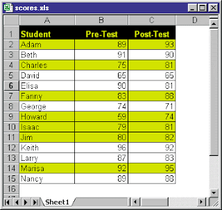
The worksheet below shows student grades on two tests. Conditional formatting highlights students who scored higher on the second test. This formatting is dynamic; if you change the test scores, the formatting adjusts automatically.

To apply conditional formatting, select range A2:C15 and choose Format, Conditional Formatting. The Conditional Formatting dialog box will appear with two input boxes. In the first box, choose Formula Is, press Tab, and enter the following formula: =$C2>$B2
Click Format and choose a format to distinguish the cells (the example uses background shading). Click OK, and the formatting will be applied.
The conditional formatting formula is evaluated for each cell in the range. The trick here is to use mixed cell references (the column references are absolute, but the row references are relative). To see how this works, activate any cell within the range and choose Format, Conditional Formatting so you can examine the conditional formatting formula for that cell. You'll find that cell A7, for example, uses this formula:=$C7>$B7.

Thanks to www.j-walk.com

Dont call it excel because now it is excellent

Its been quite a few months that myofficepower remain idle, as other projects come across the way well they did good. So it's been always a passion to talk about excel. Please keep following the new things gonna happen only on myofficepower.blogspot.com.

Work like a expert with Excel shortcut and function keys

The following lists contain CTRL combination shortcut keys, function keys, and some other common shortcut keys, along with descriptions of their functionality. For more extensive reference information on all available shortcuts and their specific uses, see Keyboard shortcuts.
CTRL combination shortcut keys
Key Description
CTRL+ ( Unhides any hidden rows within the selection.

CTRL+) Unhides any hidden columns within the selection.

CTRL+& Applies the outline border to the selected cells.

CTRL+_ Removes the outline border from the selected cells.

CTRL+~ Applies the General number format.

CTRL+$ Applies the Currency format with two decimal places
(negative numbers in parentheses).

CTRL+% Applies the Percentage format with no decimal places.

CTRL+^ Applies the Exponential number format with two decimal places.

CTRL+# Applies the Date format with the day, month, and year.

CTRL+@ Applies the Time format with the hour and minute, and AM or PM.

CTRL+! Applies the Number format with two decimal places, thousands
separator, and minus sign (-) for negative values.

CTRL+- Displays the Delete dialog box to delete the selected cells.

CTRL+* Selects the current region around the active cell (the data area
by blank rows and blank columns). In a PivotTable, it selects the entire
PivotTable report.

CTRL+: Enters the current time.

CTRL+; Enters the current date.

CTRL+` Alternates between displaying cell values and displaying formulas in
the worksheet.

CTRL+' Copies a formula from the cell above the active cell into the cell or the
Formula Bar.

CTRL+" Copies the value from the cell above the active cell into the cell or the
Formula Bar.

CTRL++ Displays the Insert dialog box to insert blank cells.

CTRL+1 Displays the Format Cells dialog box.

CTRL+2 Applies or removes bold formatting.

CTRL+3 Applies or removes italic formatting.

CTRL+4 Applies or removes underlining.

CTRL+5 Applies or removes strikethrough.

CTRL+6 Alternates between hiding objects, displaying objects, and displaying
placeholders for objects.

CTRL+7 Displays or hides the Standard toolbar.

CTRL+8 Displays or hides the outline symbols.

CTRL+9 Hides the selected rows.

CTRL+0 Hides the selected columns.

CTRL+A Selects the entire worksheet. If the worksheet contains data,

CTRL+A If the worksheet contains data,selects the current region.

Pressing CTRL+A a second time selects the entire worksheet.
When the insertion point is to the right of a function name in a formula, displays the Function Arguments dialog box.

CTRL+SHIFT+A inserts the argument names and parentheses when the insertion point is to the right of a function name in a formula.

CTRL+B Applies or removes bold formatting.

CTRL+C Copies the selected cells.

CTRL+C followed by another CTRL+C displays the Microsoft Office Clipboard.

CTRL+D Uses the Fill Down command to copy the contents and format of the topmost cell of a selected range into the cells below.

CTRL+F Displays the Find dialog box.

SHIFT+F5 also displays this dialog box, while SHIFT+F4 repeats the last Find action.

CTRL+G Displays the Go To dialog box. F5 also displays this dialog box.

CTRL+H Displays the Find and Replace dialog box.

CTRL+I Applies or removes italic formatting.

CTRL+K Displays the Insert Hyperlink dialog box for new hyperlinks or the Edit Hyperlink dialog box for selected existing hyperlinks.

CTRL+L Displays the Create List dialog box.

CTRL+N Creates a new, blank file.

CTRL+O Displays the Open dialog box to open or find a file.

CTRL+SHIFT+O selects all cells that contain comments.

CTRL+P Displays the Print dialog box.

CTRL+R Uses the Fill Right command to copy the contents and format of the leftmost cell of a selected range into the cells to the right.

CTRL+S Saves the active file with its current file name, location, and file format.

CTRL+U Applies or removes underlining.

CTRL+V Inserts the contents of the Clipboard at the insertion point and replaces any selection. Available only after you cut or copied an object, text, or cell contents.

CTRL+W Closes the selected workbook window.

CTRL+X Cuts the selected cells.

CTRL+Y Repeats the last command or action, if possible.

CTRL+Z Uses the Undo command to reverse the last command or to delete the last entry you typed.

CTRL+SHIFT+Z uses the Undo or Redo command to reverse or restore the last automatic correction when AutoCorrect Smart Tags are displayed.
Function keys
Key Description
F1
Displays the Help task pane.
CTRL+F1 closes and reopens the current task pane.
ALT+F1 creates a chart of the data in the current range.
ALT+SHIFT+F1 inserts a new worksheet.
F2
Edits the active cell and positions the insertion point at the end of the cell contents. It also moves the insertion point into the Formula Bar when editing in a cell is turned off.
SHIFT+F2 edits a cell comment.
F3
Pastes a defined name into a formula.
SHIFT+F3 displays the Insert Function dialog box.
F4
Repeats the last command or action, if possible.
CTRL+F4 closes the selected workbook window.
F5
Displays the Go To dialog box.
CTRL+F5 restores the window size of the selected workbook window.
F6
Switches to the next pane in a worksheet that has been split (Window menu, Split command).
SHIFT+F6 switches to the previous pane in a worksheet that has been split.
CTRL+F6 switches to the next workbook window when more than one workbook window is open.
Note When the task pane is visible, F6 and SHIFT+F6 include that pane when switching between panes.
F7
Displays the Spelling dialog box to check spelling in the active worksheet or selected range.
CTRL+F7 performs the Move command on the workbook window when it is not maximized. Use the arrow keys to move the window, and when finished press ESC.
F8
Turns extend mode on or off. In extend mode, EXT appears in the status line, and the arrow keys extend the selection.
SHIFT+F8 enables you to add a non-adjacent cell or range to a selection of cells by using the arrow keys.
CTRL+F8 performs the Size command (on the Control menu for the workbook window) when a workbook is not maximized.
ALT+F8 displays the Macro dialog box to run, edit, or delete a macro.
F9
Calculates all worksheets in all open workbooks.
F9 followed by ENTER (or followed by CTRL+SHIFT+ENTER for array formulas) calculates the selected a portion of a formula and replaces the selected portion with the calculated value.
SHIFT+F9 calculates the active worksheet.
CTRL+ALT+F9 calculates all worksheets in all open workbooks, regardless of whether they have changed since the last calculation.
CTRL+ALT+SHIFT+F9 rechecks dependent formulas, and then calculates all cells in all open workbooks, including cells not marked as needing to be calculated.
CTRL+F9 minimizes a workbook window to an icon.
F10
Selects the menu bar or closes an open menu and submenu at the same time.
SHIFT+F10 displays the shortcut menu for a selected item.
ALT+SHIFT+F10 displays the menu or message for a smart tag. If more than one smart tag is present, it switches to the next smart tag and displays its menu or message.
CTRL+F10 maximizes or restores the selected workbook window.
F11
Creates a chart of the data in the current range.
SHIFT+F11 inserts a new worksheet.
ALT+F11 opens the Visual Basic Editor, in which you can create a macro by using Visual Basic for Applications (VBA).
ALT+SHIFT+F11 opens the Microsoft Script Editor, where you can add text, edit HTML tags, and modify any script code.
F12
Displays the Save As dialog box.
Other useful shortcut keys
Key
Description
ARROW KEYS
Move one cell up, down, left, or right in a worksheet.
CTRL+ARROW KEY moves to the edge of the current data region (data region: A range of cells that contains data and that is bounded by empty cells or datasheet borders.) in a worksheet.
SHIFT+ARROW KEY extends the selection of cells by one cell.
CTRL+SHIFT+ARROW KEY extends the selection of cells to the last nonblank cell in the same column or row as the active cell.
LEFT ARROW or RIGHT ARROW selects the menu to the left or right when a menu is visible. When a submenu is open, these arrow keys switch between the main menu and the submenu.
DOWN ARROW or UP ARROW selects the next or previous command when a menu or submenu is open.
In a dialog box, arrow keys move between options in an open drop-down list, or between options in a group of options.
ALT+DOWN ARROW opens a selected drop-down list.
BACKSPACE
Deletes one character to the left in the Formula Bar.
Also clears the content of the active cell.
DELETE
Removes the cell contents (data and formulas) from selected cells without affecting cell formats or comments.
In cell editing mode, it deletes the character to the right of the insertion point.
END
Moves to the cell in the lower-right corner of the window when SCROLL LOCK is turned on.
Also selects the last command on the menu when a menu or submenu is visible.
CTRL+END moves to the last cell on a worksheet, in the lowest used row of the rightmost used column.
CTRL+SHIFT+END extends the selection of cells to the last used cell on the worksheet (lower-right corner).
ENTER
Completes a cell entry from the cell or the Formula Bar, and selects the cell below (by default).
In a data form, it moves to the first field in the next record.
Opens a selected menu (press F10 to activate the menu bar) or performs the action for a selected command.
In a dialog box, it performs the action for the default command button in the dialog box (the button with the bold outline, often the OK button).
ALT+ENTER starts a new line in the same cell.
CTRL+ENTER fills the selected cell range with the current entry.
SHIFT+ENTER completes a cell entry and selects the cell above.
ESC
Cancels an entry in the cell or Formula Bar.
It also closes an open menu or submenu, dialog box, or message window.
HOME
Moves to the beginning of a row in a worksheet.
Moves to the cell in the upper-left corner of the window when SCROLL LOCK is turned on.
Selects the first command on the menu when a menu or submenu is visible.
CTRL+HOME moves to the beginning of a worksheet.
CTRL+SHIFT+HOME extends the selection of cells to the beginning of the worksheet.
PAGE DOWN
Moves one screen down in a worksheet.
ALT+PAGE DOWN moves one screen to the right in a worksheet.
CTRL+PAGE DOWN moves to the next sheet in a workbook.
CTRL+SHIFT+PAGE DOWN selects the current and next sheet in a workbook.
PAGE UP
Moves one screen up in a worksheet.
ALT+PAGE UP moves one screen to the left in a worksheet.
CTRL+PAGE UP moves to the previous sheet in a workbook.
CTRL+SHIFT+PAGE UP selects the current and previous sheet in a workbook.
SPACEBAR
In a dialog box, performs the action for the selected button, or selects or clears a check box.
CTRL+SPACEBAR selects an entire column in a worksheet.
SHIFT+SPACEBAR selects an entire row in a worksheet.
CTRL+SHIFT+SPACEBAR selects the entire worksheet.
If the worksheet contains data, CTRL+SHIFT+SPACEBAR selects the current region. Pressing CTRL+SHIFT+SPACEBAR a second time selects the entire worksheet.
When an object is selected, CTRL+SHIFT+SPACEBAR selects all objects on a worksheet.
ALT+SPACEBAR displays the Control menu for the Excel window.
TAB
Moves one cell to the right in a worksheet.
Moves between unlocked cells in a protected worksheet.
Moves to the next option or option group in a dialog box.
SHIFT+TAB moves to the previous cell in a worksheet or the previous option in a dialog box.
CTRL+TAB switches to the next tab in dialog box.
CTRL+SHIFT+TAB switches to the previous tab in a dialog box.

Ms Excel 2003 Logo Screen

Microsoft Excel startup screen.

Believe it or not : Excel Dominating the Globe

We at My Office power just posting about the scope of Ms Excel and Ms Word and all other Ms office applications. We have just began to let you know how important is it to be aware of market demands today. Perhaps Excel has taken place in major IT industries providing international software soloutions. Oracle the name is enough we need not to elaborate about this name. Oracle is now has launched software applications in Ms Excel globally. And as we have been speaking about Excel Dominance in the global industry since its inception day by day we are updating about the hottest and latest on Excel and all other Ms Office applications. My blog is not just upto posting it is something more. You send your comments on our blog we will explore our knowledge for you. As always your truly , yours own, myofficepower.blogspot.

My Office Power: Excel plays a major role in IT industries

My Office Power: Excel plays a major role in IT industries

Excel plays a major role in IT industries

Big IT firms in India like Wipro has implemented Excel for e-procurement business providing e-tendering services to its clients from governmental organisations.

Know about security of your files

You must be keeping important data in your excel sheets may be it is about financial, official statistics data or whatever it may be very confidential, you never know if some one get access to it and got stolen from your system, then what will you do ?

You should keep it securely in your system by means of protecting your document feature of Ms Office.

If you don't know about this feature of Ms Office learn about this today...........


If you want to protect a Excel file protect it by applying password to the particular file,
follow the link below to know how you can safegaurd your documents.

LEARN HOW TO PROTECT YOUR DOCUMENTS

See how Excel can reduce your mental stress

Microsoft Excel (full name Microsoft Office Excel) is a spreadsheet program written and distributed by Microsoft for computers using the Microsoft Windows operating system and for Apple Macintosh computers. It features an intuitive interface and capable calculation and graphing tools which, along with aggressive marketing, have made Excel one of the most popular microcomputer applications to date. It is overwhelmingly the dominant spreadsheet application available for these platforms and has been so since version 5 in 1993 and its bundling as part of Microsoft Office.

Yes Excel has got the power to reduce your mental stress by easing your complex calculaions.

Why Excel is so powerful because Excel is a software where a spreadsheet is a rectangular table (or grid) of information, often financial information. The word came from "spread" in its sense of a newspaper or magazine item (text and/or graphics) that covers two facing pages, extending across the center fold and treating the two pages as one large one. The compound word "spread-sheet" came to mean the format used to present bookkeeping ledgers — with columns for categories of expenditures across the top, invoices listed down the left margin, and the amount of each payment in the cell where its row and column intersect—which were traditionally a "spread" across facing pages of a bound ledger (book for keeping accounting records) or on oversized sheets of paper ruled into rows and columns in that format and approximately twice as wide as ordinary paper.

more.....