Excel is excellent and lets see how it helps you using this drop down list features !
If you don't want to risk an item being miss-typed in a cell, drop down lists are an ideal solution. So These lists display all of the available choices to the user so that they can click on their preference. Excel allows you to place two different types of drop down list on your worksheet - either a validation list or a form object.
A validation drop down list
 These lists are contained within a cell on your worksheet and the drop down arrow (to the right of the cell) does not appear unless the cell is selected. To add a list to a worksheet place the cursor in the required cell and then selectData Validation Settings. In the dialog box select 'Allow: List' and ensure the 'In-cell dropdown' box is ticked. The source data refers to a range of cells containing the selection of options. If you use the mouse to point to a range of cells (e.g. H12:H15), they must normally be contained on the same worksheet. If however you have named the range of cells (e.g. '=ConsNames') containing your data, it can be anywhere in the workbook.
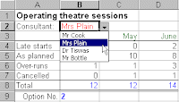
In the example (right) the list has been placed in cell B2. Having selected 'Mrs Plain' the formulae in the table (B3:D8) lookup values in a range of data and summarise it. The consultant name can be referred to by the cell name (B2). If you wish to know the position of the selected item within the original range of options (i.e. the four names), an additional formula is needed. In cell B9, the formula =MATCH(B2, H12:H15, 0) determines that Mrs Plain is the second item in the list.
If you don't want to risk an item being miss-typed in a cell, drop down lists are an ideal solution. So These lists display all of the available choices to the user so that they can click on their preference. Excel allows you to place two different types of drop down list on your worksheet - either a validation list or a form object.
A validation drop down list
 These lists are contained within a cell on your worksheet and the drop down arrow (to the right of the cell) does not appear unless the cell is selected. To add a list to a worksheet place the cursor in the required cell and then selectData Validation Settings. In the dialog box select 'Allow: List' and ensure the 'In-cell dropdown' box is ticked. The source data refers to a range of cells containing the selection of options. If you use the mouse to point to a range of cells (e.g. H12:H15), they must normally be contained on the same worksheet. If however you have named the range of cells (e.g. '=ConsNames') containing your data, it can be anywhere in the workbook.
In the example (right) the list has been placed in cell B2. Having selected 'Mrs Plain' the formulae in the table (B3:D8) lookup values in a range of data and summarise it. The consultant name can be referred to by the cell name (B2). If you wish to know the position of the selected item within the original range of options (i.e. the four names), an additional formula is needed. In cell B9, the formula =MATCH(B2, H12:H15, 0) determines that Mrs Plain is the second item in the list.
Using a combo box or a list box

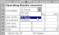
These are independent objects (or controls) that can be placed onto a worksheet and are not contained within a cell as such. The example (left) contains a combo box but your choice of object can depend on the amount of space on your worksheet and the number of options.
To obtain these controls you must open the Forms toolbar (View Toobars Forms). Then click on either of the list buttons and drag an outline for the object on your worksheet. To instruct the new control where to find it's source data, right click on it, then choose Format Controlfrom the short menu. On the 'Control' tab of the dialog box, enter the range of cells containing the list options. The 'Cell Link' refers to a cell where you wish the list box to place a numeric value representing selected item. In the example above cell B21 is linked and indicates that the third list item was selected. You cannot refer directly to the value in the list box, but the option number in your worksheet cell is automatically updated to reflect any change in the control object.
To determine the actual name of the selected item (i.e. Dr Tiswas), use a formula such as =OFFSET(H11, B21, 0) where H11 is the cell immediately above the options list and B21 contains the option value. (Click here for details about the OFFSET function).
To determine the actual name of the selected item (i.e. Dr Tiswas), use a formula such as =OFFSET(H11, B21, 0) where H11 is the cell immediately above the options list and B21 contains the option value. (Click here for details about the OFFSET function).
credit:www.meadinkent.co.uk
